library(tidyverse)
library(scales)

source(here::here("src", "R", "x_theme.R"))

# ------------------------------------------------------------
# DATA REQUIREMENTS
# ------------------------------------------------------------
# Your data should be a long-format dataframe with:
#   - zone:        character/factor, zone label (for faceting)
#   - op_temp:     numeric, operative temperature [°C]
#   - occupied:    integer, 0/1 occupancy indicator
#   - season:      factor, "Winter" / "Spring" / "Summer" / "Autumn"
#   - run_avg_oat: numeric, prevailing mean outdoor air temperature [°C]
# ------------------------------------------------------------

# SAMPLE DATA (replace with your own hourly timeseries)
set.seed(42)
make_zone <- function(base, amp_annual, amp_diurnal, sd_noise, label) {
  expand.grid(doy = 1:365, hour_day = 0:23) %>%
    as_tibble() %>%
    mutate(
      month_num   = as.integer(format(as.Date(doy - 1, origin = "2025-01-01"), "%m")),
      annual      = -cos(2 * pi * doy / 365),
      diurnal     = sin(pi * hour_day / 12 - pi / 6),
      op_temp     = base + amp_annual * annual + amp_diurnal * diurnal + rnorm(n(), 0, sd_noise),
      run_avg_oat = 15 + 7 * annual,
      occupied    = as.integer(hour_day >= 7 & hour_day <= 22),
      season      = factor(case_when(
        month_num %in% c(12, 1, 2) ~ "Winter",
        month_num %in% c(3, 4, 5)  ~ "Spring",
        month_num %in% c(6, 7, 8)  ~ "Summer",
        TRUE                        ~ "Autumn"
      ), levels = c("Winter", "Spring", "Summer", "Autumn")),
      zone = label
    )
}

op_temp_long <- bind_rows(
  make_zone(21, 5.5, 2.5, 0.6, "Living zone"),
  make_zone(20, 8.0, 3.5, 1.0, "Garage zone"),
  make_zone(22, 11.0, 5.0, 1.5, "Attic zone")
) %>%
  mutate(zone = factor(zone, levels = c("Living zone", "Garage zone", "Attic zone")))

op_occ <- op_temp_long %>% filter(occupied > 0)

# ASHRAE 55 adaptive comfort bands per season
ashrae_bands <- op_temp_long %>%
  group_by(season) %>%
  summarise(mean_pma = mean(run_avg_oat, na.rm = TRUE), .groups = "drop") %>%
  mutate(
    ashrae_upper = 0.31 * mean_pma + 21.3,
    ashrae_lower = 0.31 * mean_pma + 14.3,
    x    = as.integer(season),
    xmin = x - 0.45,
    xmax = x + 0.45
  )

# ------------------------------------------------------------
# PLOT
# ------------------------------------------------------------
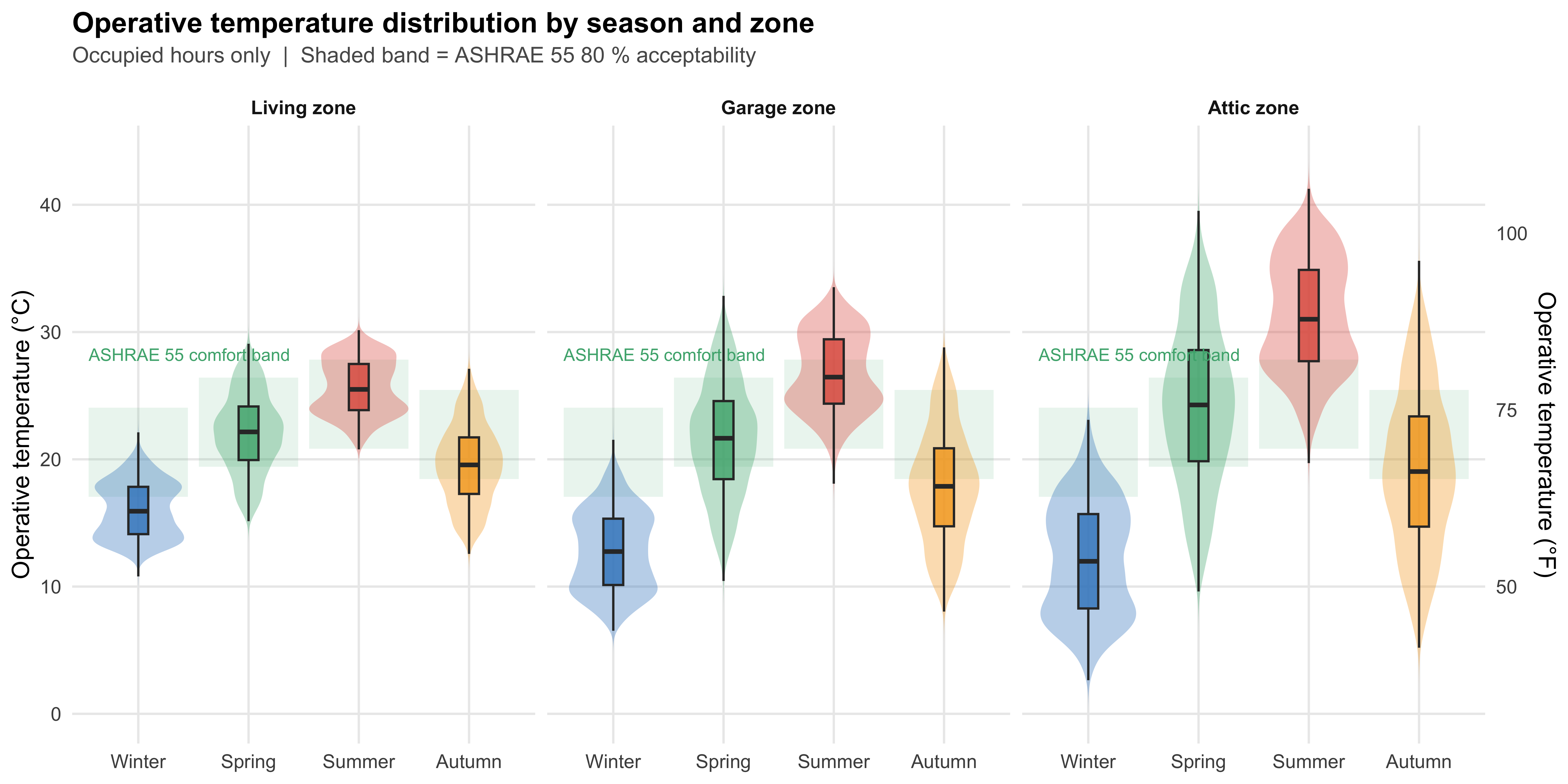
ggplot(op_occ, aes(x = season, y = op_temp, fill = season)) +
  geom_rect(
    data = ashrae_bands,
    aes(xmin = xmin, xmax = xmax, ymin = ashrae_lower, ymax = ashrae_upper),
    inherit.aes = FALSE, alpha = 0.12, fill = "#4CAF7D"
  ) +
  geom_violin(alpha = 0.35, colour = NA, trim = FALSE) +
  geom_boxplot(width = 0.18, outlier.size = 0.4, alpha = 0.8) +
  annotate("text",
           x = 0.55, y = max(ashrae_bands$ashrae_upper) + 0.4,
           label = "ASHRAE 55 comfort band",
           size = 2.8, colour = "#4CAF7D", hjust = 0) +
  scale_y_continuous(
    name     = "Operative temperature (°C)",
    sec.axis = sec_axis(~ . * 9 / 5 + 32, name = "Operative temperature (°F)")
  ) +
  scale_fill_manual(values = c(
    Winter = "#3A85C6", Spring = "#4CAF7D",
    Summer = "#E05C4B", Autumn = "#F5A623"
  )) +
  facet_wrap(~zone, nrow = 1) +
  labs(
    title    = "Operative temperature distribution by season and zone",
    subtitle = "Occupied hours only  |  Shaded band = ASHRAE 55 80 % acceptability",
    x = NULL
  ) +
  theme_ep() +
  theme(legend.position = "none")