# ============================================================
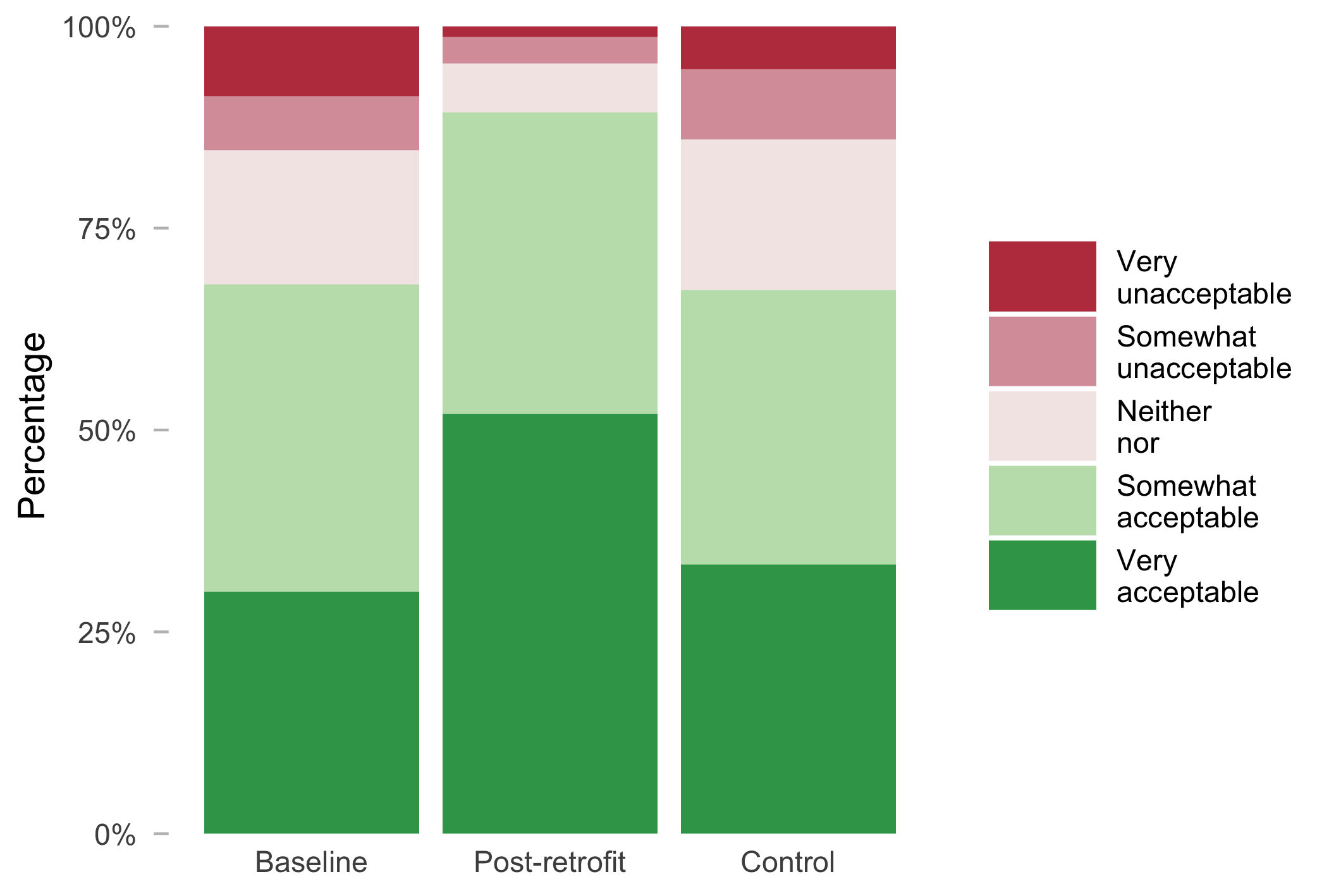
# THERMAL ACCEPTABILITY DISTRIBUTION PLOT
# ============================================================
# This script creates a 100% stacked bar chart showing the
# distribution of thermal acceptability votes across survey conditions.
#
# Required packages: tidyverse, scales
# Color palette: source from src/R/x_theme.R
# ============================================================
library(tidyverse)
library(scales)
# Load color palette
source(here::here("src", "R", "x_theme.R"))
# ------------------------------------------------------------
# DATA REQUIREMENTS
# ------------------------------------------------------------
# Your data should be a dataframe with:
# - survey_id: factor identifying survey condition (e.g., "Baseline", "Post-retrofit")
# - thermal_acceptability: factor with levels c("Very unacceptable", "Somewhat unacceptable", "Neither nor", "Somewhat acceptable", "Very acceptable")
#
# Example structure:
# survey_id thermal_acceptability
# <fct> <fct>
# Baseline Somewhat acceptable
# Baseline Very acceptable
# Post-retrofit Neither nor
# ...
# ------------------------------------------------------------
# SAMPLE DATA (replace with your own data)
# This demonstrates the required data structure
acceptability_levels <- c(
"Very unacceptable", "Somewhat unacceptable",
"Neither nor",
"Somewhat acceptable", "Very acceptable"
)
survey_ids <- c("Baseline", "Post-retrofit", "Control")
set.seed(123)
survey <- purrr::map_dfr(
survey_ids,
~ tibble::tibble(
survey_id = .x,
thermal_acceptability = sample(
acceptability_levels,
size = 150,
replace = TRUE,
prob = case_when(
.x == "Baseline" ~ c(0.05, 0.10, 0.20, 0.35, 0.30),
.x == "Post-retrofit" ~ c(0.02, 0.05, 0.10, 0.33, 0.50),
.x == "Control" ~ c(0.06, 0.10, 0.20, 0.34, 0.30),
TRUE ~ rep(1/5, 5)
)
)
)
) %>%
mutate(
survey_id = factor(survey_id, levels = survey_ids),
thermal_acceptability = factor(thermal_acceptability, levels = acceptability_levels)
)
# ------------------------------------------------------------
# PLOT CODE
# ------------------------------------------------------------
ggplot(survey %>% drop_na(thermal_acceptability),
aes(x = survey_id, fill = thermal_acceptability)) +
geom_bar(position = position_fill(reverse = TRUE), show.legend = TRUE) +
scale_y_continuous(labels = percent, expand = expansion(mult = c(0, 0.01))) +
scale_fill_manual(values = acceptability_palette, labels = label_wrap_gen(width = 9), drop = FALSE) +
labs(y = "Percentage") +
theme_minimal(base_size = 7) +
theme(
legend.position = "right",
legend.direction = "vertical",
legend.title = element_blank(),
panel.grid.major = element_blank(),
panel.grid.minor = element_blank(),
axis.title.x = element_blank(),
axis.ticks.y = element_line(color = "grey", linewidth = 0.25),
axis.ticks.x = element_blank(),
axis.ticks.length = unit(1, "mm")
) +
guides(
fill = guide_legend(
reverse = TRUE,
ncol = 1,
byrow = TRUE,
label.position = "right",
keywidth = unit(7.5, "mm"),
keyheight = unit(5, "mm"),
label.hjust = 0,
label.vjust = 0.5
)
)